Note: This post was back-ported from LessWrong. You can find the original here.
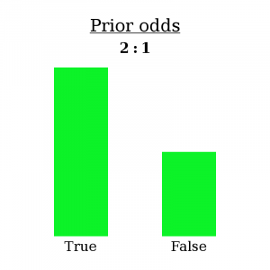
Let’s say you have a belief — I’ll call it “B” for “belief” — that you would assign 2:1 odds to. In other words, you consider it twice as likely that B is true than that B is false. If you were to sort all possible worlds into piles based on whether B is true, there would be twice as many where it’s true than not.
Then you make an observation O, which you estimate to have had different probabilities depending on whether B is true. In fact:
- If B is true, then O had a 1/8 chance of occurring.
- If B is false, then O had a 3/4 chance of occurring.
In other words:
- O occurs in 1/8 of the worlds where B is true.
- O occurs in 3/4 of the worlds where B is false.
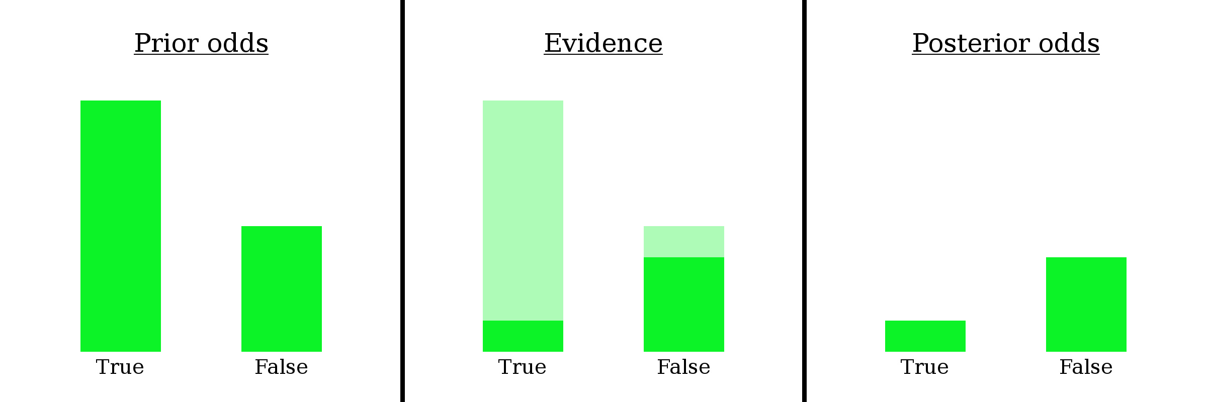
We know you’re in a world where O occurred — you just saw it happen! So let’s go ahead and fade out all the worlds where O didn’t occur, since we know you’re not in one of them. This will slash the “B is true” pile of worlds down to 1/8 of its original size and the “B is false” pile of worlds down to 3/4 of its original size.
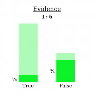
Why did I write Evidence: 1:6 at the top? Let’s ignore that for a second. For now, it’s safe to throw away the faded-out worlds, because, again, we now know they aren’t true.
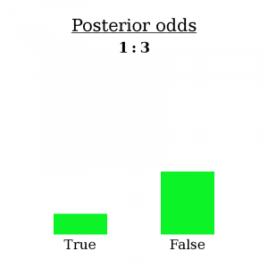
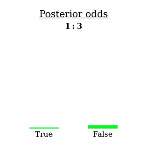
I’m going to make a bold claim: having made observation O, you have no choice but to re-asses your belief B as having 1:3 odds (three times as likely to be false than true).
How can I say such a thing? Well, initially you assigned it 2:1 odds, meaning that you thought there were twice as many possible worlds where it was true than where it was false. Having made observation O, you must eliminate all the worlds where O doesn’t happen. As for the other worlds, if you considered them possible before, and O doesn’t contradict them, then you should still consider them possible now. So there is no wiggle room: an observation tells you exactly which worlds to keep and which to throw away, and therefore determines how the ratio of worlds changes — or, how the odds change.
What about “Evidence: 1:6”?
Well, first notice that it doesn’t really matter how many worlds you’re considering total — what matters is the ratio of worlds in one pile to the other. We can write 2:1 odds as the fraction 2/1. The numerator represents the “B is true” worlds and the denominator represents the “B is false” worlds. Then, when you see the evidence, the numerator gets cut down to 1/8 of its initial size, and the denominator gets cut down to 3/4 of its initial size.
We can write this as an equation:
(2 ∗ 1/8) / (1 * 3/4) = 1/3
Now notice something else: it also doesn’t matter what the actual likelihood of observation O is in each type of world. All that matters is the ratio of likelihoods of O between one type of world and the other. O could just as well have been exactly 10 times less likely in both scenarios…
(2 ∗ 1/80) / (1 * 3/40) = 1/3
…and our final odds come out the same.
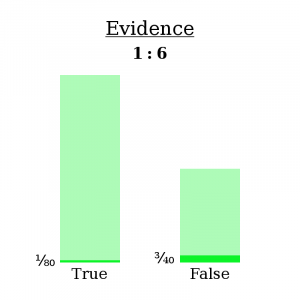
That’s why we write the evidence as 1:6 — because only the ratio matters.
This — the fact that each new observation uniquely determines how your beliefs should change, and the fact that this unique change is to multiply by the ratio of likelihoods of the observation — is Bayes’ Theorem. If it all seems obvious, good: clear thinking renders important theorems obvious.
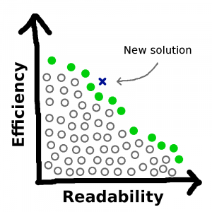
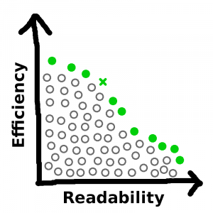
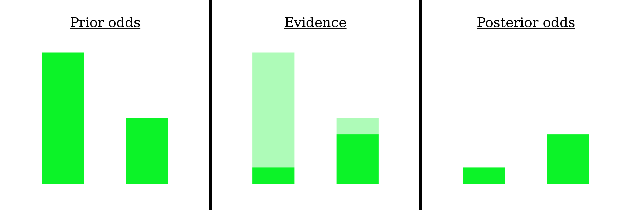
For your viewing pleasure, here’s a combined picture of the three important diagrams.

And here’s a version without the numbers and here’s a version where the bars aren’t even labeled.
An example
On the LessWrong version of this post, user adamzerner suggested I add a concrete example. I’m happy to oblige!
Example: Mahendra has been found dead in his home, killed by a gunshot wound. Police want to know: was this a suicide or a homicide?
The first step is to establish your prior; in other words, what odds [homicide : suicide] do you assign this case right off the bat?
Well, according to Vox, about 40% of gun-related deaths are homicides and 60% are suicides. The number has varied a bit throughout the years, but let’s go ahead and use this figure. A 40%/60% chance equates to 2:3 odds — for every two homicides by gun, there are three suicides by gun. This is called the base rate, and it will serve as our prior odds.
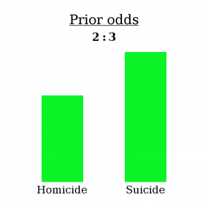
It’s worth repeating that what you see above represents the fact that, if you sorted all possible worlds into piles based on Mahendra’s cause of death, you would see three in the “suicide” pile for every two in the “homicide” pile. (It’s okay if there are other modes of death under consideration too, such as “accident” — the same logic would still apply! For simplicity, I’ll just use these two.)
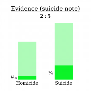
After a bit of investigation, a some evidence has turned up — a suicide note! Open and shut case, right?
Think again. Some murderers are smart — they’ll plant a fake suicide node at the scene of the crime to cover their tracks. I couldn’t find an exact statistic, but let’s say about 1/10 murderers think to do this.
Also, not every suicide has a note. In fact, Wikipedia reports that only about 1/4 of suicides include a note.
In other words:
- If Mahendra’s death was a homicide, there was a 1/10 chance of finding a note.
- If Mahendra’s death was a suicide, there was a 1/4 chance of finding a note.
So now, let’s follow the same process as before.
Here’s the math bit:
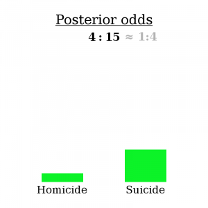
(2 ∗ 1/10) / (3 * 1/4) = 4/15
So, as expected, finding a suicide note makes the “homicide” explanation less likely — 4:15 odds compared to 2:3 odds, or about a 79% chance of suicide compared to a 60% chance initially.
However, be aware that this isn’t because most suicides include a note. In fact, most suicides don’t include a note. The reason it makes suicide more likely is that even fewer homicides include a note. It’s not true that “most suicides have a note”, but it is true that “suicides are more likely to produce a note than homicides are”. That’s what makes for proper bayesian evidence.